User Manual
Starting MEAFS
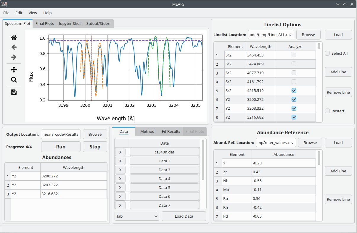
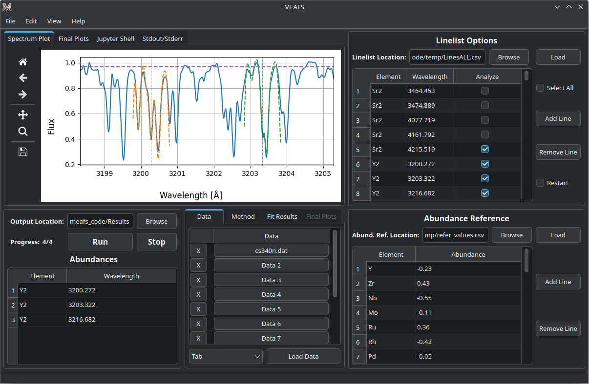
View mode
MEAFS can adapt to the system settings and can be used in the Light or Dark mode, as bellow.
Loading a line-list
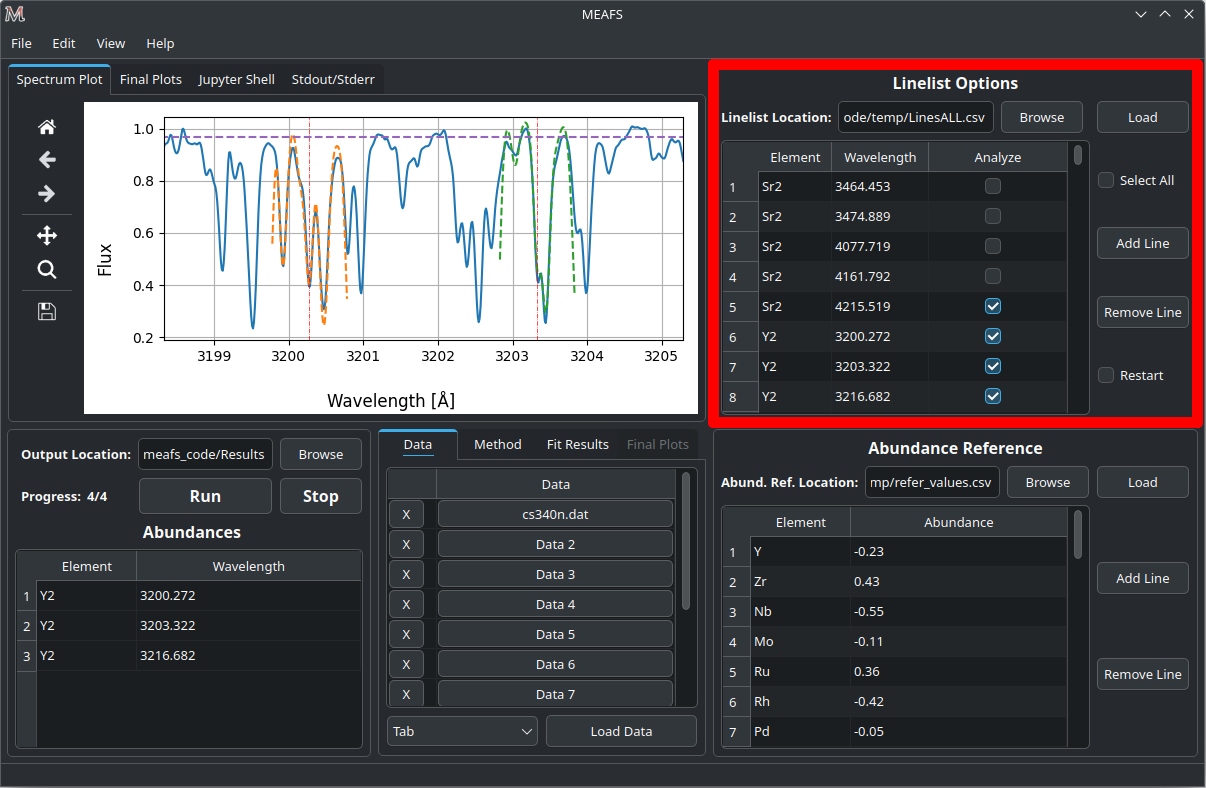
MEAFS operates in a line-list based workflow. Every single measurement, needs to be listed in the line-list.
There are three columns in the line-list field:
Element |
The element and order of the corresponded wavelength. |
Wavelength |
The wavelength intended to be analyzed. |
Analyze |
A checkbox if this wavelength should or should not be analyzed. |
Obs: rows beginning with # in the CSV file are ignored.
The checkbox Select All can check or uncheck all the Analyze column checkboxes.
The Restart checkbox change the behavior of MEAFS in how it will read the line-list. If it is unchecked, MEAFS will ignore lines that are already in the found_values.csv file (see Analyzing Results). Otherwise, if it is checked, MEAFS will fit all selected lines and overwrite them in the results file.
If a line that is selected is out of the range of any spectrum data, this line will be skipped.
Loading abundance references

The Abundance Reference table works in the same way as the Linelist table. Except for that there are only two columns:
Element |
The element that the abundance refers to. |
Abundance |
The reference abundance for this element. |
The reference abundance will be used as the first guess for the optimization method (Equivalent Width excluded).
Loading spectra data
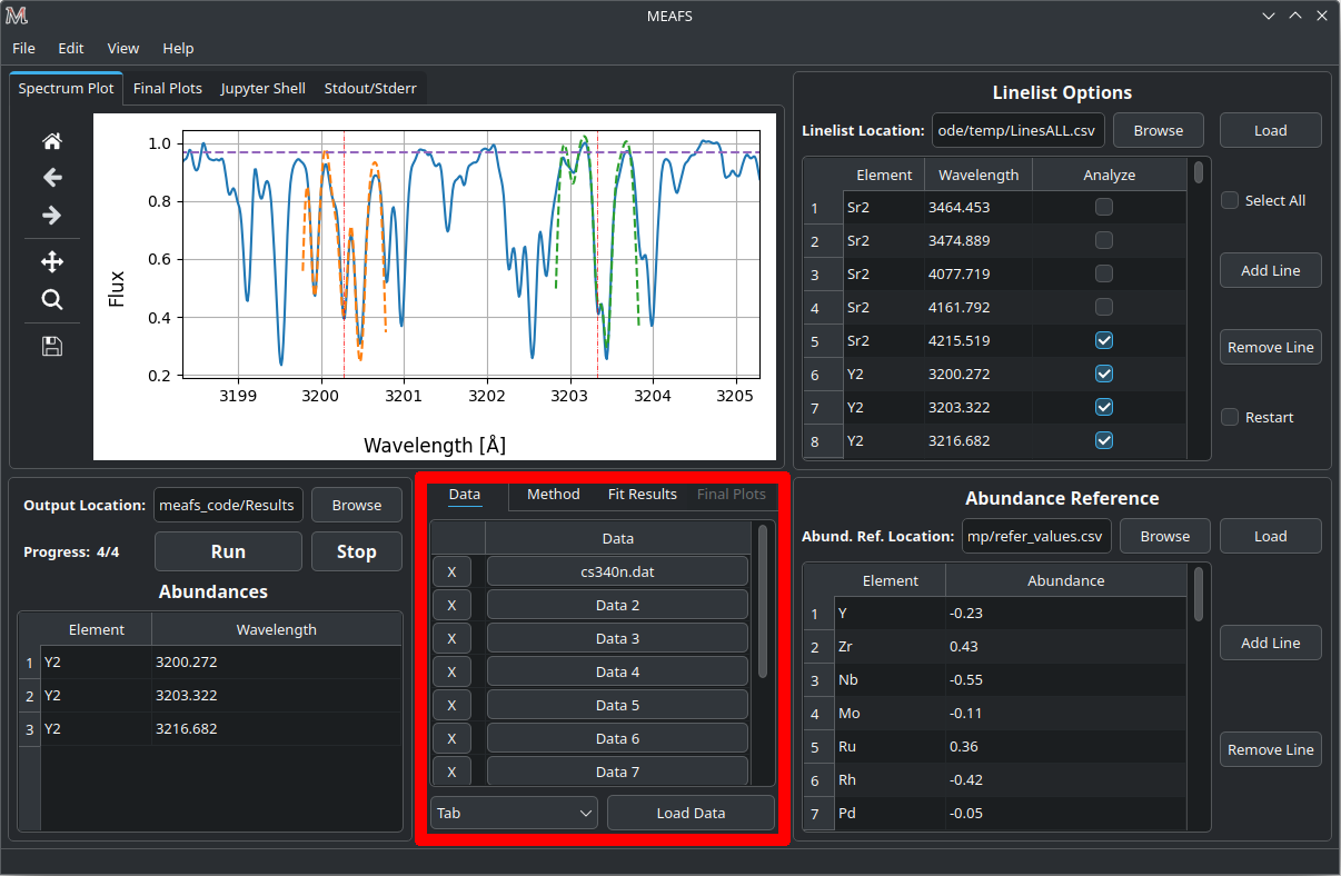
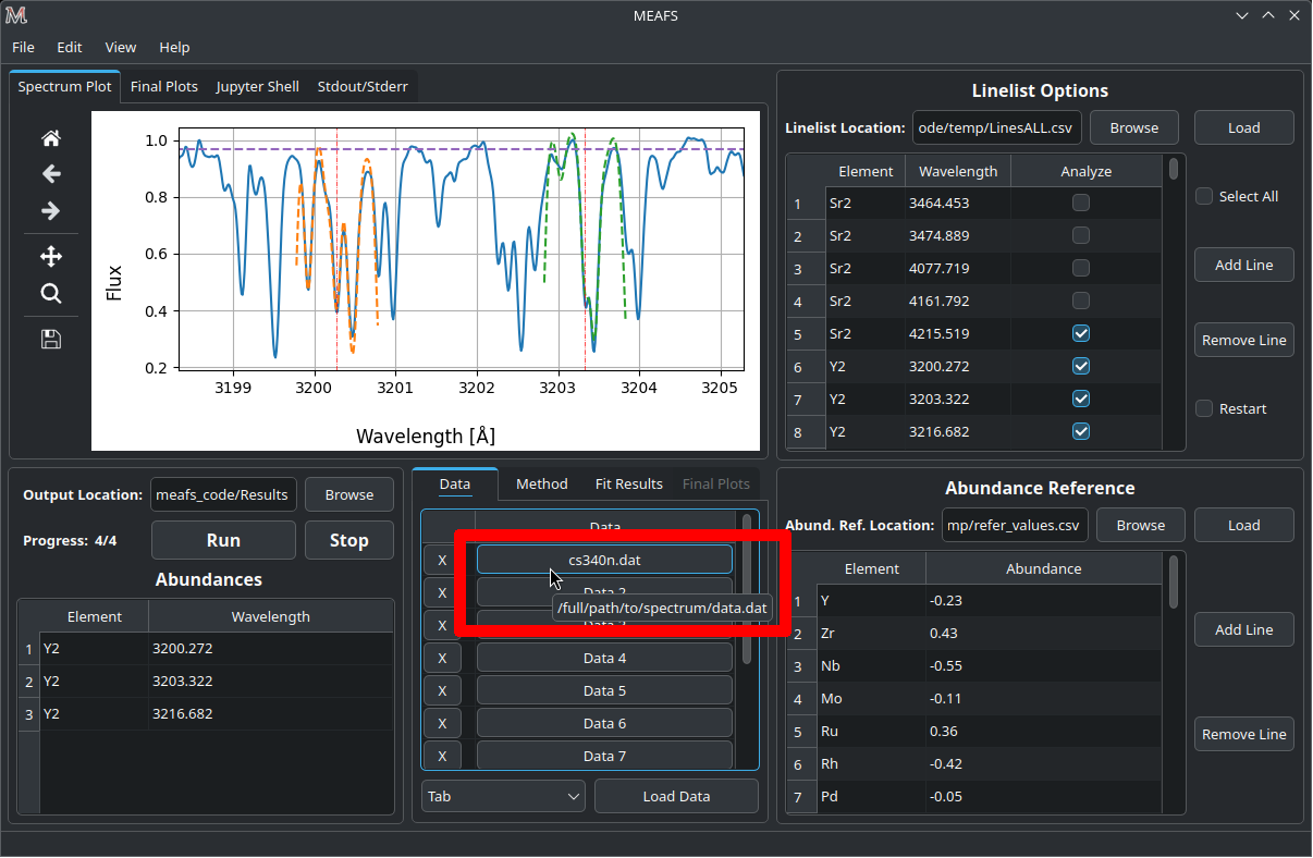
Auto: automaticaly try to determine the delimiter type. This will work with multiple files with different delimiters;
Tab/Multiple spaces: multiple files need to have the same delimiter type;
Comma: multiple files need to have the same delimiter type.
Obs: rows beginning with # in the CSV file are ignored.
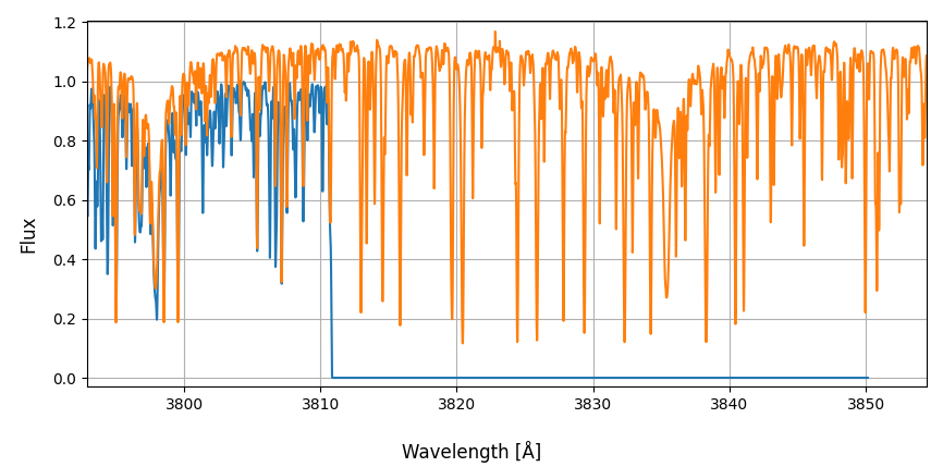
Attention: For overlapping spectra, the fit will be processed only for the first spectrum in the Data table order. Moreover, it is advised not to upload spectra with edge effects (e.g., zero flux; see image below). Otherwise, if allocated first in the Data table, MEAFS will attempt to fit the non-existing data in the first spectrum instead of the one with real data.
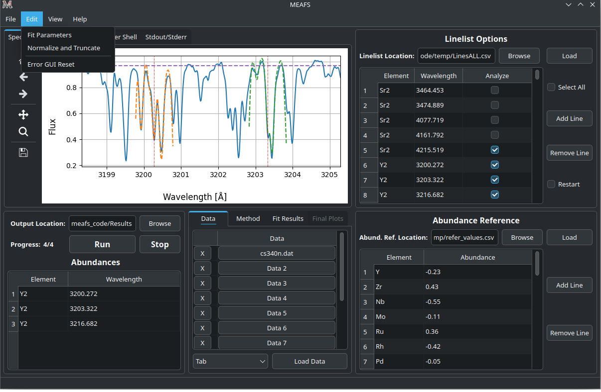
Normalization and Truncation
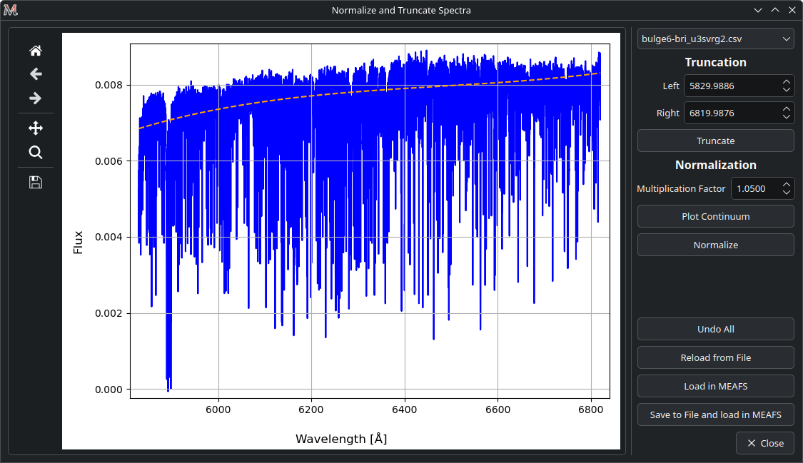
After a successful spectrum load, it is possible to truncate and normalize each spectrum within MEAFS. To do this, go to Edit > Normalize and Truncate. This will open a new window where it is possible to select each previously loaded spectrum.
To truncate a spectrum, simply set the minimum and maximum desired range and click Truncate;
To normalize, first adjust the multiplication factor, plot the continuum, and then click Normalize.
The Undo All button reverts all changes that have not yet been loaded in MEAFS. While the Reload from File button reloads the spectrum from its file.
The changes made are not automaticaly applied to MEAFS. To apply them, click either Load in MEAFS or
Save to File and load in MEAFS buttons. The latter creates a new spectrum file in the same directory
as the original, with the same name plus the suffix _norm. If the location is unavailable, the file
is created in the Output Location (see Full run).
When the Save to File and load in MEAFS is triggered, the original file reference is replaced by the new
one. This means that the loaded file in MEAFS will now point to the new _norm file. At this stage,
the Reload from File button will no longer work since the file name has changed. To use the original
file again, return to the main window and load it manually (either by replacing the new _norm file or
by using an empty slot).
Selecting the method

Currently, in the Methods tab, these methods to generate a synthetic spectrum can be selected:
Method |
Description |
|---|---|
Eq. Width |
Uses a Gaussian, Lorentzian or Voigt profile to create the spectrum. |
TurboSpectrum |
Uses the TurboSpectrum (Plez B, 2012) to create the spectrum. |
Equivalent Width
For this method, it can be used three different functions:
Gaussian:
(1)\[f(x) = a \cdot \exp\left[\frac{-(x - b)^2}{c \cdot \sqrt{2 \cdot \pi}}\right] + d\]Lorentzian:
(2)\[g(x) = a \cdot \exp\left[\frac{c}{\pi \cdot ((x - b)^2 + c^2)}\right] + d\]Voigt:
(3)\[h(x) = a \cdot f(x) \cdot g(x) + d\]With \(f(x)\) being the (1) and \(g(x)\) being the (2).
In this case, the values of \(a\) and \(d\) for both \(f(x)\) and \(g(x)\) are \(=0\).
The first guess for the method fit can also be defined:
Convolution |
Parameter \(c\) |
Depth |
Parameter \(a\) |
TurboSpectrum

TurboSpectrum2019 can be found here: https://github.com/bertrandplez/Turbospectrum2019
TurboSpectrum_NLTE (not tested) can be found here: https://github.com/bertrandplez/Turbospectrum_NLTE
In the first run of MEAFS, it will be created a folder called modules in
the root directory of MEAFS (this directory can be found by typing in a
terminal meafs -h). It is advised (but not mandatory) to add the
TurboSpectrum module in this folder.
Full run

After filling all the other tables and selecting the desired synthetic spectrum method, the results folder location needs to be defined. click Browse and select the folder.
Obs: If the folder name is not “Results”, MEAFS will create another folder inside the select one with this name.
To run, just click Run to start the fit of all selected lines and Stop to end the run in the middle.
Obs: the Stop button will finish the current line before it takes effect.
While running, the GUI will be frozen, being actualized only few times after each line. At each actualization, the plot area and the tab Fit Results will show the last successful fit.
At the end of each line, MEAFS save the results. In case of an unwanted interruption, open MEAFS again and use the menu option File > Open Abundances… and it will populate the plot and the results table (see Open old results (not sessions)).
Fit parameters
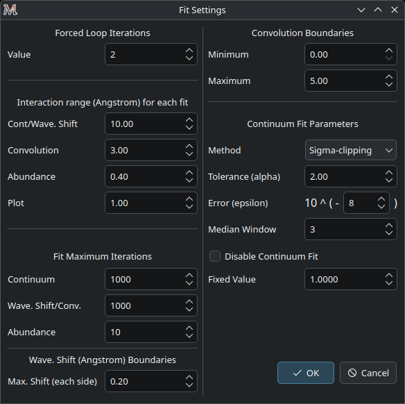
There are several options to change how the fit is done. This menu is located in Edit > Fit Parameters.
Change it with caution, since this can drastically modify the results.
Forced Loop Iterations
There is one parameter that determines how many iterations the main fit routine will run.
The main goal here is to have the first fit with no guesses and a second one using the results of the previous one as a start point. That is why the default value is 2.
Interaction range (Å) for each fit
For each fit, the spectrum will be restrained to a certain range. The parameters here determine this range.
For example, the plot range, by default, plots a range of \(1 Å\) (centered in the wavelength of the line and \(0.5 Å\) for each side). But let’s suppose that it is needed to see a line in the same plot that is \(1.2 Å\) apart from the line that has been fitted. Then, the range for the plot can be set for \(3 Å\).
For the abundance, if a wide range is used, the \(\chi^2\) may not be fully minimized, since the abundance in the synthetic spectrum only changes the lines of that specific element. Therefore, a smaller range may benefit the minimization. The resolution of the spectrum can have a huge impact on this.
Fit Maximum Iterations
This sets a limit to the maximum number of iterations that each method can use. This can have an impact in how long does it take to fit a line and if it will actually be fitted or the method will be ended before it achieves a satisfactory result.
Wave. Shift (Å) Boundaries
The wavelength shift fit sometimes can try to fit a line that is next to the desired one, especially for crowded regions. To prevent this of happening, the boundaries of the fit can be defined.
Convolution Boundaries
The convolution parameters are very specific for each spectrum and, if the user already have a guess of what it is, the constrains can be fixed.
Continuum Fit Parameters
There are 3 different methods to fit the continuum:
Sigma-clipping
Chebyshev
Simple Average
And also an option to disable the fit at all and use a fixed value for the continuum. The default behavior is to use the Sigma-clipping method.
The Sigma-clipping is expected to provide the best performance for a normalized and metal-rich spectrum. Thus, it is advised to normalize all spectra before running the fit. See Normalization and Truncation.
See Check continuum fit for a way to verify if the chosen method and its parameters are satisfactory or not.
Sigma-clipping
The Sigma-clipping continuum level method described in Sánchez-Monge, 2018: STATCONT: A statistical continuum level determination method for line-rich sources.
To summarize it, it is a iteration method that exclude outliers to find the median and the standard deviation of the flux axis and uses these values for the continuum and its errors, respectively.
The process involves two parameters that determine how the method will be handled:
\(\alpha\) |
Is a weight for the standard deviation that determines which outliers will be ignored or not. The expression is:
\[\mu \pm \alpha \sigma\]
Where \(\mu\) is the median of the array and \(\sigma\) is the standard deviation. The values that are above of this limit, are considered outliers, therefore are excluded from the array. |
\(\epsilon\) |
Determines the relative error of the iteration process by applying:
\[\frac{\sigma_{old}-\sigma}{\sigma} \leq \epsilon\]
Where \(\sigma\) is the current standard deviation of the array and the \(\sigma_{old}\) is from the previous iteration. |
Chebyshev
The Chebyshev method is as described in Astropy Chebyshev1D. It is an univariate Chebyshev series defined as:
With \(T_i (x)\) being the corresponding Chebyshev polynomial of the 1st kind.
The input parameter is the Median Window, which is defined here.
Simple Average
This method simply calculates the mean of the flux, no input parameters are necessary. It has poor performance with metal-rich stars.
Disable Continuum Fit
It is also possible to completely disable the fit of the continuum and replace it by a fixed linear value. Note that this value will be applied for all lines, and no individual line fit will be made.
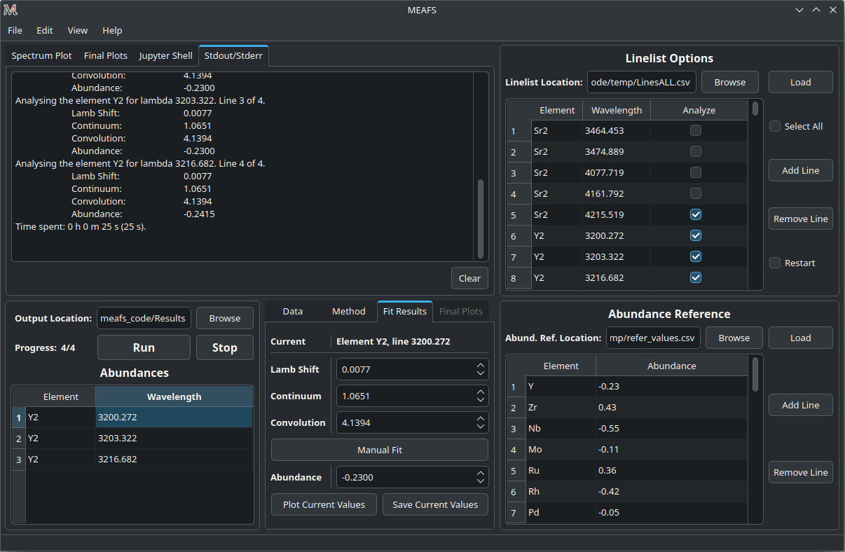
Preliminary view of the results
After the full run, the lines that are selected in the line-list will appear in the Abundances table if they are in the range of the spectrum (lines that are not in the range of any spectrum will be skipped).
Clicking in one row of this table will select the line and the results of the fit of this line will be shown in the Fit Results tab.
Also, all the results are saved in the found_values.csv file (see Analyzing Results).
The plot
The plot area shows all loaded spectra and all fitted lines. Once one line is clicked in the results table, the plot will focus on that specific line.
It is possible to modify the range, pam, save, zoom in and out using the Matplotlib toolbar next to the plot.
To show the full spectrum range, there is a button in the menu option View > Change Plot to full spectrum range. But there is also a keyboard shortcut for that: Ctrl+Shift+V.
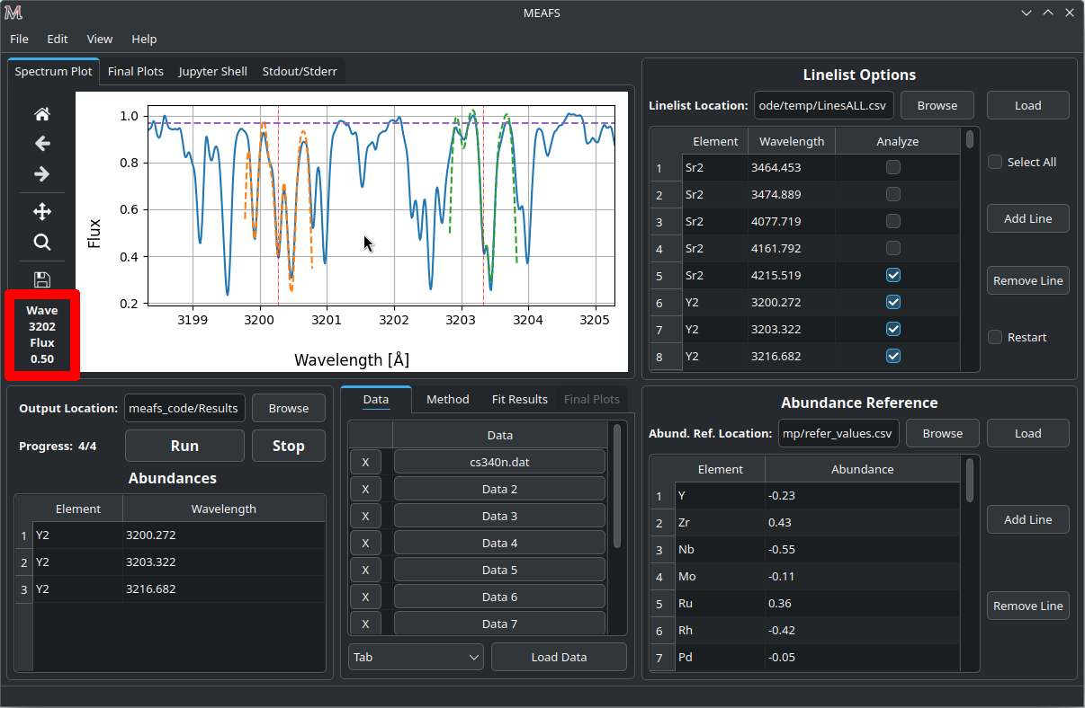
When the mouse pointer is on top of the plot, the axis values appear in the toolbar, like in the image below:
Sometimes the plot can be very crowded, you may want to clean the lines fit and other draws. It is possible to this by clicking in the menu View > Clear Spectrum Plot.
Then, you can use the option Open old results (not sessions) to load again only the last fitted lines.
Check continuum fit
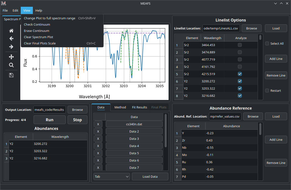
It is possible to plot the continuum in the menu option View > Check Continuum and erase it with Erase Continuum button in the same submenu. Note that it is not needed to have the continuum plotted in the figure to proceed with the fit, this is just to check if the method and its parameters are good or not as described in Continuum Fit Parameters.
Although it is possible to check and adjust the continuum parameters in a global scale, each line will have its own local continuum fit (with the selected parameters).
Fit only abundance run
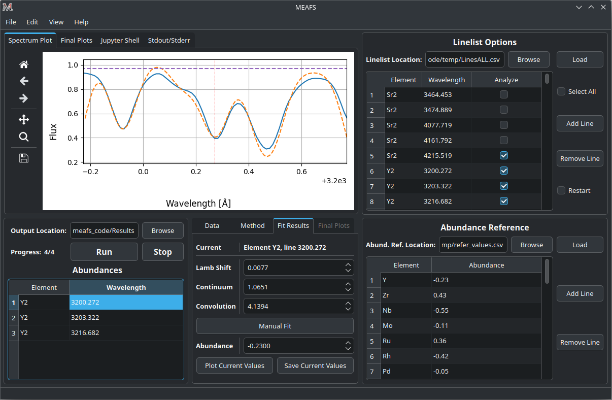
After a full run, the lines selected will appear in the results table and can be selected. As showed in Preliminary view of the results, the fit results can be found in the Fit Results tab.
In this tab, it is possible to manually change the Lamb Shift, Continuum and Convolution values and press the Manual fit button. Every time this button is pressed, it will run a fit only for the abundance using the values that are written in these three parameters above.
The Lamb Shift is given in Ångstroms, the Continuum is given in the spectrum Flux unit and the Convolution in given in the line FWHM.
After this run, the new abundance and the modified parameters will be written in the found_values.csv file. To restore the originals values, it is needed to run the fit again (only for the desired line) with the Restart option enabled.
No fit run
As described in Fit only abundance run, in the Fit Results tab, it is possible to modify the Lamb Shift, Continuum and Convolution values, however it is also possible to change the abundance value and Plot Current Values in the plot. This will not save the results in the found_values.csv, for that press Save Current Values.
Analyzing Results
All the results are saved in the found_values.csv file, under the directory previously chosen for the results. This file has the following columns:
Element |
Corresponding element of this line. |
Lambda (Å) |
Wavelength in Ångstroms. |
Lamb Shift |
Wavelength shift in Ångstroms for this line. |
Continuum |
Continuum value for this line in the spectrum Flux unit. |
Convolution |
Convolution value for this line the line FWHM. |
Refer Abundance |
Reference abundance of the element. |
Fit Abundance |
Found abundance for this line. |
Differ |
Absolute difference of the reference and the fitted abundance. |
Chi |
Minimized \(\chi^2\) of the abundance fit. |
Equiv Width Obs (Å) |
Equivalent width of the observed spectrum. |
Equiv Width Fit (Å) |
Equivalent width of the synthetic fitted spectrum. |
Not only that, MEAFS can also create three different types of plots that helps extracting the abundances and other parameters from the fit.
These plots can be created and viewed in the Final Plots tabs.
Attention: the Final Plots tab next to the Fit Results tab can only be accessed when the Final Plots tab next to Spectrum Plot tab is selected.
The visualization of these plots in MEAFS is only a scaled image of the actual file created. In order to view the full image without any quality loss, open the image file in the previously defined directory for the results.
Resizing GUI upon viewing images
When any image is added into MEAFS, the software will block the scale of the image. This blocks resizing the GUI into smaller sizes. If necessary, to unlock the scale go to View > Clear Final Plots Scale.
Lines Plot
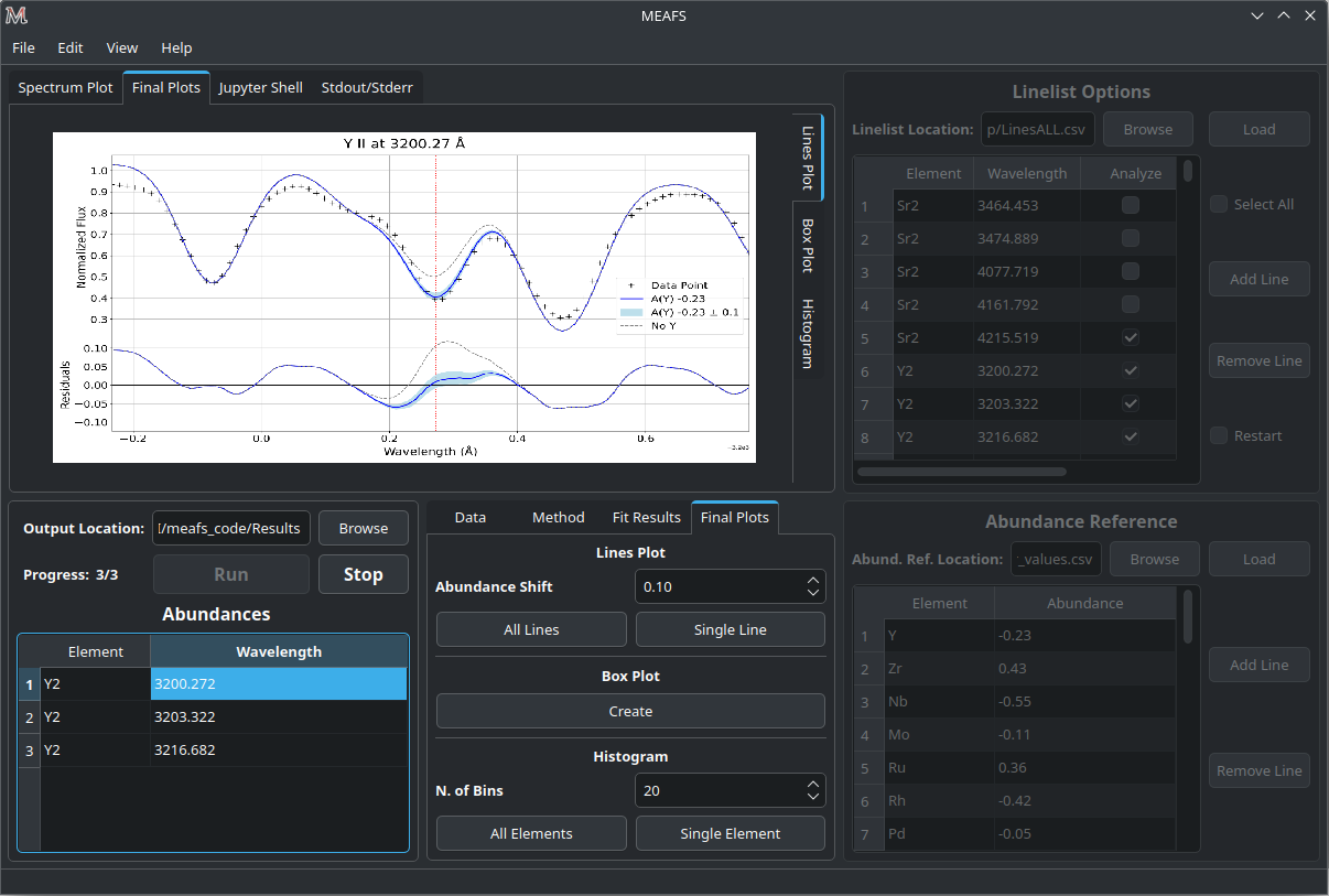
MEAFS is able to create fancy plots for all lines that are in the abundances table.
The plot lines are:
Data Points |
Spectrum data. |
Best Fit |
Synthetic Spectrum with best fit abundance. |
Abundance Shift |
Synthetic Spectrum with abundance increased and decreased by a defined value to create a shaded light blue area around the best fit. |
Zero Abundance |
Synthetic Spectrum with no abundance. |
Residuals |
Absolute residuals of data points and best fit abundance. |
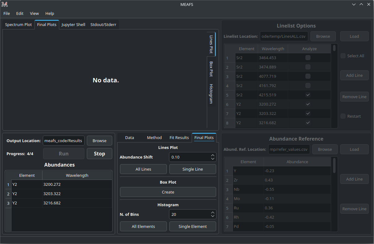
The region of the abundance shift can be set in the Final Plots tab.
It is possible to create plots for all lines at once in the All Lines button, or select one line in the table and click Single Line button.
When you select any line in the table, MEAFS will search for the file to plot it, if there is any old file in the right folder with the right name, it will be showed. If there is not, a “No data.” label will appear.
Box Plot

The box plot can be generated under the Create button in the Final Plots tab. MEAFS will create a full box plot with all the elements and lines available in the abundance table.
The plot will show the mean, median, maximum, minimum, confidence level (25% and 75% quartiles) and outliers abundances for each element accordingly with the fit results.
Histogram
Two types of histograms can be created:
Abundances Histogram;
Difference Histogram.
The number of bins for the histograms can be defined in the Final Plots tab and, like the Lines Plot, the All Elements button will generate it for all elements at once and the Single Element button will do it only for the element selected in the abundance table.
Also, like the Lines Plot, by clicking in any line in the abundance plot, MEAFS will load the file or show “No Data.” label instead.
Abundances Histogram
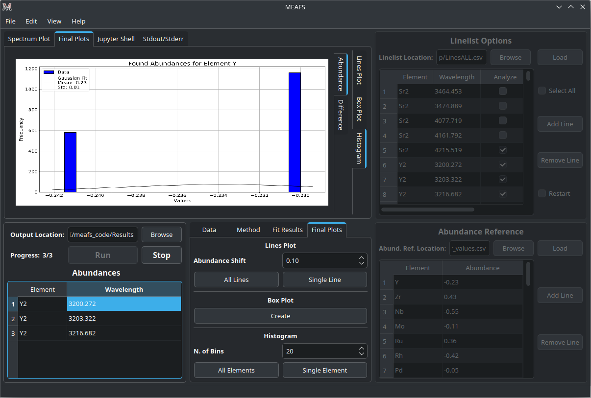
The Abundance Histogram consists in a simple histogram showing the distribution of the abundances for the specific element.
Difference Histogram
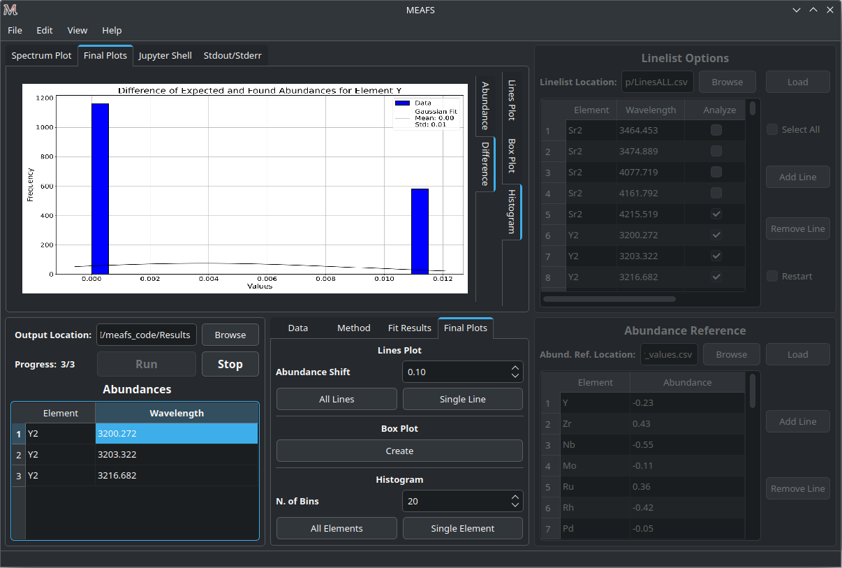
The Difference Histogram consists in showing the distribution of the absolute value of the difference between the fit abundance and the reference abundance.
Jupyter Shell
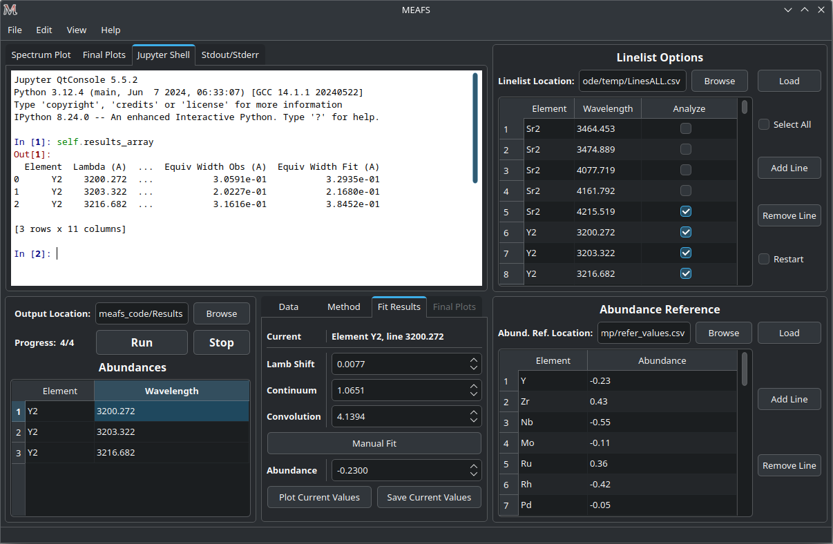
The Jupyter Shell tab provides access to the MEAFS session with all the variables and functions available. It can be useful for more advanced user or for debug. See Package Overview for the list of variables and functions.
Stdout and Stderr
All print functions and errors of the code are redirected to the Stdout/Stderr tab. Use it for debug and/or follow up the fit process.
It is possible to clear the Stdout/Stderr text area by pressing the Clear button.
Errors while running the fit
In case of errors while running a fit, some widgets of the GUI may be frozen. To unlock them, go to the menu option Edit > Error GUI Reset.
Save and open sessions
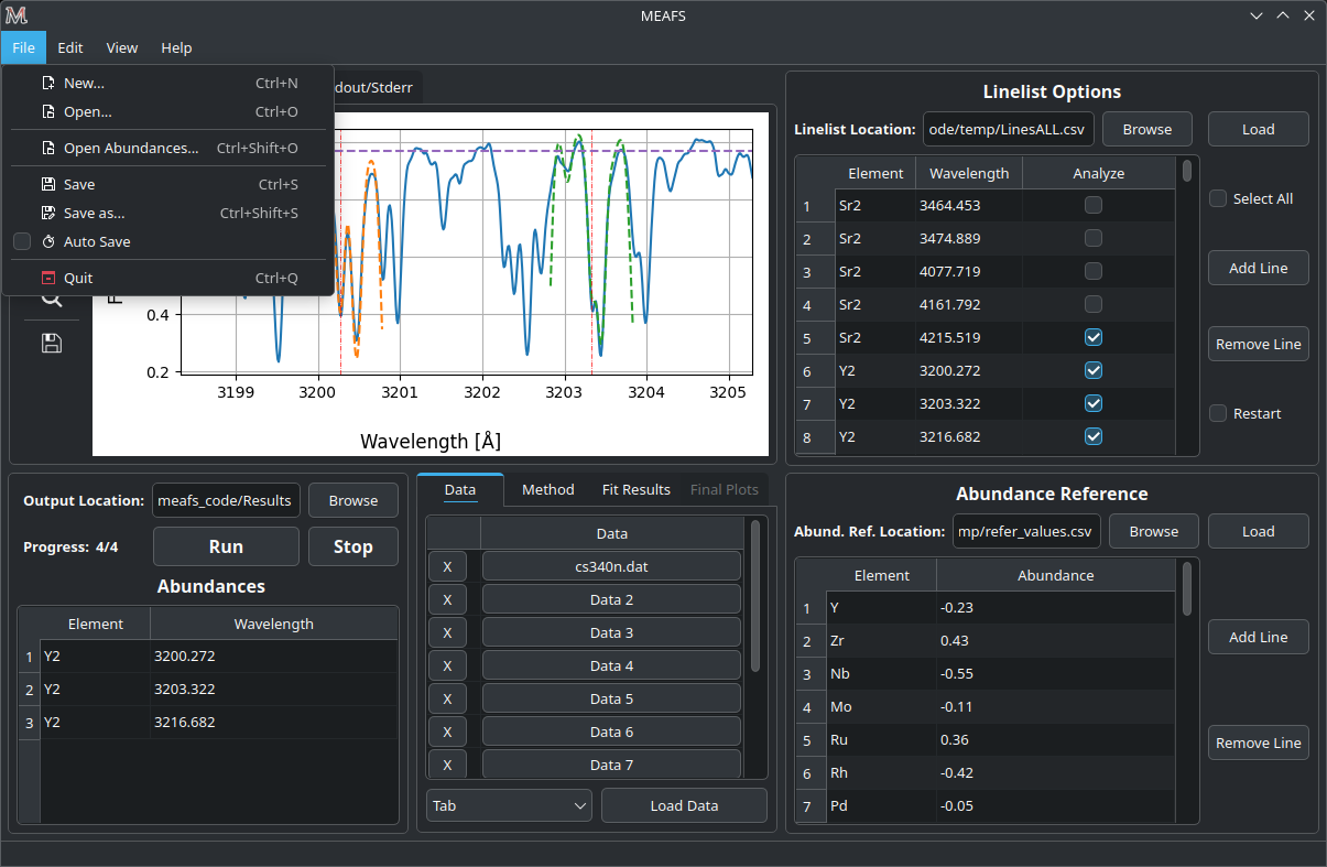
MEAFS uses the dill library to create sessions of the current loaded values. Sessions can be saved and opened, or a new empty one can be created. Note that creating a new session will erase all current values, save them before doing this.
Auto Save
There is an Auto Save function that will save a session every 60 seconds. Not only that, every time the MEAFS is closed, it will trigger to save the session if this feature is on.
To enable or disable this function, go to File > Auto Save.
These sessions are saved at the MEAFS root directory (this directory can be
found by typing in a terminal meafs -h). The file names for each type of
auto save can be checked below:
File Name |
Description |
|---|---|
auto_save.pkl |
Session saved every 60 seconds. |
auto_save_last.pkl |
Session saved when MEAFS is closed. |
To open the last 60 seconds auto save file, go to a terminal and type:
meafs -s
And to open the last closed session, type:
meafs -l
Open old results (not sessions)
Help Section
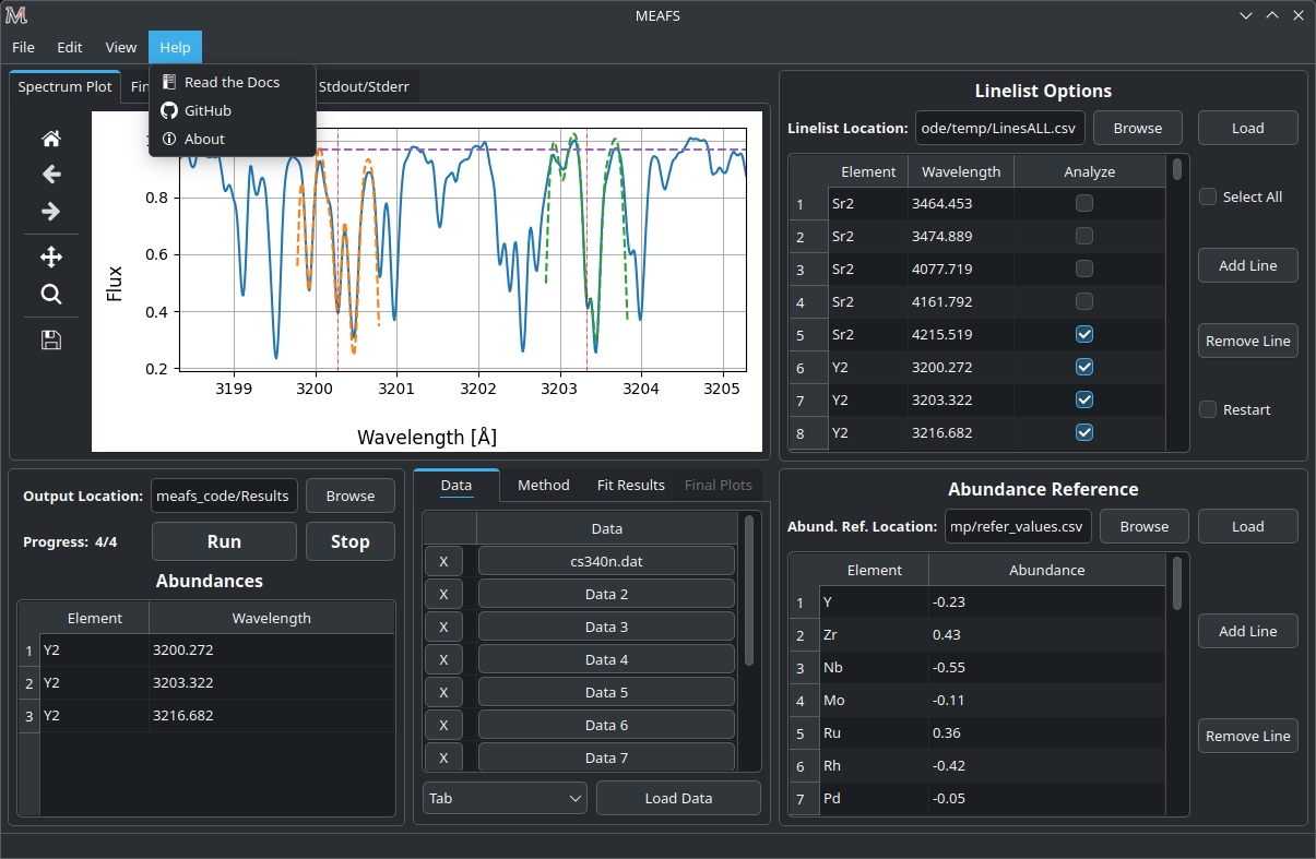
There is a Help menu in the menu bar with links to this Read the Docs and the GitHub page.
If the information you need or a bug you are facing is not listed in this manual, you can open an issue or ask for help in GitHub Issues.